Step-by-step explanation:
Hello!
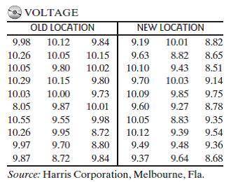
You have the information about voltage readings at an old and a new manufacturing location obtained remotely.
a, b and c in the attachment.
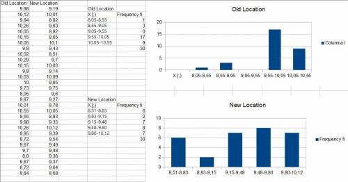
Histograms for a and c:
To construct a frequency histogram you have to first arrange the data for both locations in a frequency table. For this, I'm going to determine 5 class interval for each location. To do so you need to calculate the width of the intervals. First, you calculate the range of the variable and then you have to divide it by the number of intervals you want to do.
Old location: Range= 10,55-8,05= 2,5 → Class width: 2,5/5= 0,5
New Location: Range= 10,12-8,51= 1,61 → Class width: 1,61/5= 0,322
Starting from the minimum value you add the calculated width and create the intervals:
Old Location:
8,05-8,55
8,55-9,05
9,05-9,55
9,55-10,05
10,05-10,55
New Location
8,51-8,83
8,83-9,15
9,15-9,48
9,48-9,80
9,80-10,12
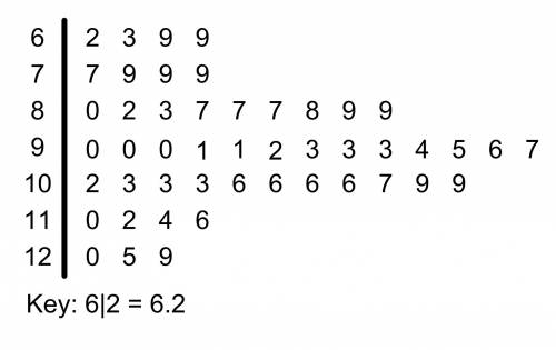
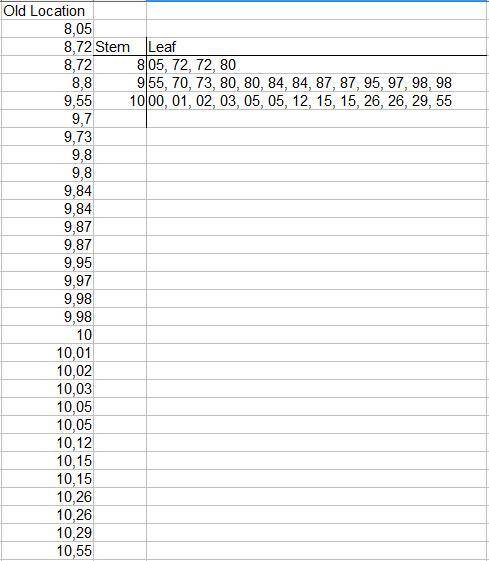
Stem and Leaf diagram for b:
To construct this diagram first I've ordered the data from leat to greatests. Then I've used the integer to form the stem 8,- 9.- and 10.- and the decimals are placed in the leafs of the diagram.
Comparing it to the histogram and stem and leaf diagram for the readings of the Old Location, the histogram stem, and leaf diagram show better where most of the readings lie.
d.
Comparing both histograms, it looks like the readings in the new location are more variable than the readings in the old location but more uniformly distributed. I would say that the readings in the new location are better than the readings in the old location.
e.
To calculate the mean you have to apply the following formula:
X[bar]= (∑xi'fi)/n
X[bar]OLD=(∑xi'fi)/n= (8.3*1+8.8*3+9.3*0+9.8*17+10.3*9)/30= 294/30= 9.8
X[bar]NEW=(∑xi'fi)/n= (8.67*6+8.99*2+9.315*7+9.64*8+9.96*7)/30= 282.045/30= 9.4015≅9.40
First you have to calculate the position of the median:
For both data sets the PosMe= 30/2=15
Now you arrange the data from least to highest and determine wich observation is in the 15th position:
Old Location
8,05 , 8,72 , 8,72 , 8,8 , 9,55 , 9,7 , 9,73 , 9,8 , 9,8 , 9,84 , 9,84 , 9,87 , 9,87 , 9,95 , 9,97 , 9,98 , 9,98 , 10 , 10,01 , 10,02 , 10,03 , 10,05 , 10,05 , 10,12 , 10,15 , 10,15 , 10,26 , 10,26 , 10,29 , 10,55
MeOLD= 9.97
New Location
8,51 , 8,65 , 8,68 , 8,78 , 8,82 , 8,82 , 8,83 , 9,14 , 9,19 , 9,27 , 9,35 , 9,36 , 9,37 , 9,39 , 9,43 , 9,48 , 9,49 , 9,54 , 9,6 , 9,63 , 9,64 , 9,7 , 9,75 , 9,85 , 10,01 , 10,03 , 10,05 , 10,09 , 10,1 , 10,12
MeNEW= 9.43
The mode is the observation with more absolute frequency.
To determine the mode on both data sets I'll use the followinf formula:
Md= Li + c [Δ₁/(Δ₁+Δ₂)]
Li= Lower bond of the interval with most absolute frequency (modal interval)
c= amplitude of the modal interval
Δ₁= absolute frequency of the modal interval minus abolute frequency of the previous interval
Δ₂= absolute frequency of the modal interval minus the absolute frequency of the next interval
Modal interval OLD
9,55-10,05
Δ₁= 17-0= 17
Δ₂= 17-9= 8
c= 0.5
Li= 9.55
MdOLD= 9.55 + 0.5*[17/(17+8)]= 9.89
Modal interval NEW
9,48-9,80
Δ₁= 8-7= 1
Δ₂= 8-7= 1
c= 0.32
Li= 9.48
MdNEW= 9.48+0.32*[1/(1+1)]= 9.64
f.
OLD
Mean 9.8
SE 0.45
X= 10.50
Z= (10.50-9.8)/0.45= 1.56
g.
NEW
Mean 9.4
SE 0.48
X=10.50
Z= (10.50-9.4)/0.48=2.29
h. The Z score for the reading 10.50 for the old location is less than the Z score for the reading 10.50 for the new location, this means that the reading is closer to the mean in the old location than in the new location.
The reading 10.50 is more unusual for the new location.
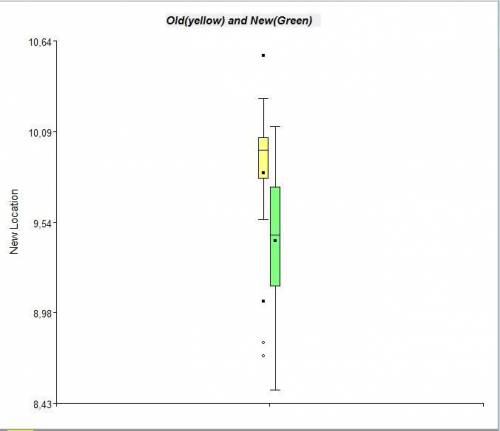
i. and k. Boxplots attached.
There are outliers for the readings in the old location, none in the readings for the new location.
j. To detect outliers using the Z- score you have to "standardize every value of the data set using the corresponding values of the mean and standard deviation. Observations that obtained a Z-score greater than 3 or less than -3 are outliers.
The data set for the new location has no outliers, To prove it I've calculated the Z-scores for the max and min values:
Min: Z=(8.51-9.4)/0.48= -1.85
Max: Z=(10.12-9.4)/0.48= 1.5
The records for the old location show, as seen in the boxplot, outliers:
To find them I'll start calculating values of Z from the bottom and the top of the list until getting a value Z≥-3 and Z≤3
Bottom:
1) 8,05 ⇒ Z=(8.05-9.8)/0.45= -3.89
2) 8,72 ⇒ Z= (8.72-9.8)/0.45= -2.4
Top
1) 10,55⇒ Z= (10.55-9.8)/0.45= 1.67
m. As mentioned before, the distribution for the new location seems to be more uniform and better distributed than the distribution for the old location. Both distributions are left-skewed, the distribution for the data of the old location is severely affected by the presence of outliers.
I hope this helps!

 5
5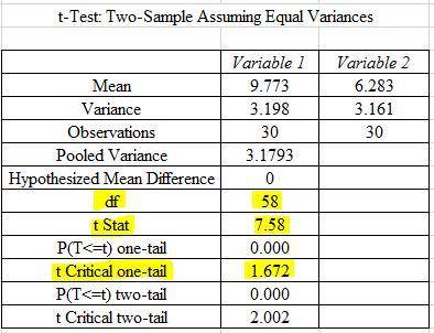
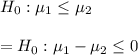 versus

 if
if 
 Summing up the samples given , we have 331.6
 : Average EER = 9
 : Average ≠ 9

 , where 'n' is the number of data
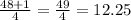 rounded down to 12
 on the diagram which is 8.7